In my previous tutorial I have described the steps for a land cover classification using the Semi-Automatic Classification Plugin for QGIS. The classification result is a raster file; however, certain spatial analyses require the vector format.
This post is about the conversion of a land cover classification from raster to vector format (that is a shapefile) using QGIS. In addition, I will describe some useful functions for the refinement of the output file.
The following instructions are for QGIS 1.8; also, the installations of the SEXTANTE plugin, and SAGA are required (for information about software installation see here). The SEXTANTE plugin is a framework that allows QGIS to execute the functions of other programs, such as SAGA GIS.
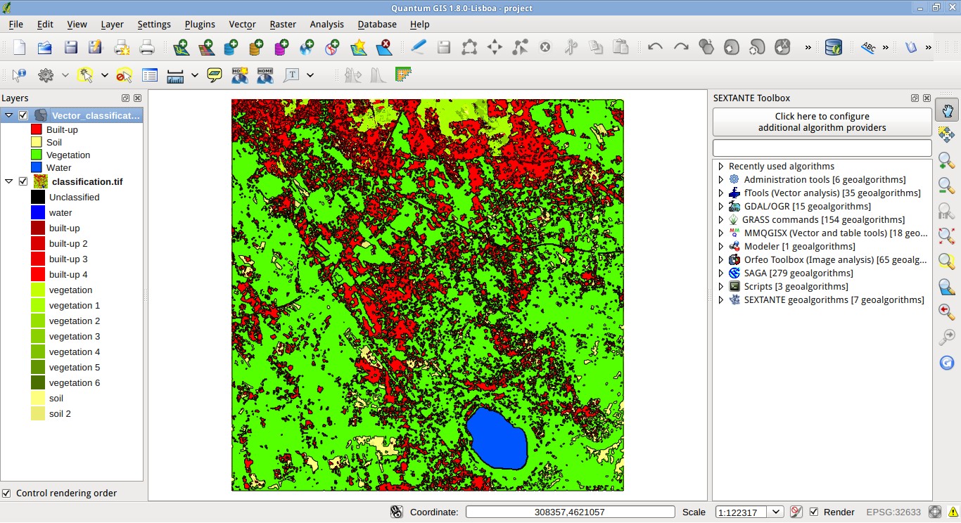
- Open the classification raster in QGIS. You can download a sample classification (the result of the previous tutorial and its QGIS style) from here.

- The classification process requires the collection of several ROIs (and several classes), therefore the land cover classification may have some redundant classes. For example, in my previous tutorial we have identified several vegetation classes that can be grouped in one vegetation class.It is possible to reclassify the classification according to the list of classes we want, producing a new raster classification (a temporary file).
- From the menu "Analysis" activate the "Sextante toolbox"; navigate to "SAGA" > "Grid - Tools" and double click "Reclassify Grid Values";
- We are going to create a table with the reclassification values: under "Grid" select "classification.tif"; under "method" select "[2] simple table";

- Under "Lookup table" click the button "..." to open the "Fixed Table" interface; here, we are going to type the reclassification values; the lookup table has 3 columns: "minimum", "maximum", and "new". Minimum and maximum define the reclassification range for the new value.We define 4 classes plus the "Unclassified" value, as in the following table (class description in italics);
- Click twice the button "Add row", in order to have five records, and fill the table as in the following image; click "OK" when done;
| minimum | maximum | new | |
|---|---|---|---|
| 0 | 0 | 0 | Unclassified |
| 1 | 1 | 1 | Water |
| 2 | 5 | 2 | Built-up |
| 6 | 12 | 3 | Vegetation |
| 13 | 14 | 4 | Soil |

- Select the operator "[1] min <= value <= max";
- Click "OK" and after a few seconds the new classification will be loaded in QGIS (as a temporary file);
- Double click on the new classification in the "Layer" panel; select the "Style" tab and beside "Color map" choose "Colormap"; select the "Coloramp" tab and click 5 times "Add entry"; change the "Value", "Color" and "Label" fields according to our reclassification table, as in the following image;
- Click the button "Export color map to file" (the floppy icon), and save the file as "classes.txt" (this file will be useful later);
- Click the button "Save Style" and save this color map as "class_style.qml"; then click"OK" to view the map colors.


- It can be useful to eliminate isolated pixels for the purpose of reducing noise, or producing a more homogeneous landscape (consequently, the final shapefile will have less polygons and a smaller file size). We are going to apply one of the SAGA filters (i.e. the "Majority filter"*) on the reclassification raster, and to produce a new filtered raster.The "Majority filter" allows for the identification of the predominant or most frequent occurring classification value, in a defined neighborhood of cells (i.e. matrix), assigning that value to the central cell (from the "SAGA User Guide" that you can download from here).
- From the "Sextante toolbox" navigate to "SAGA" > "Grid - Filter" and double click "Majority filter";
- Under "Grid" select the reclassification raster (its name begins with "sagareclassifygridvalues"); we leave the default "Search Mode" (i.e. "[0] Square") and the "Radius" (i.e. 1) parameters, which mean that a 3 x 3 filter matrix is used;
- Under "Threshold [Percent]" set the parameter to 66 (it means that at least 6 pixels having the same value are needed to change the central cell value in the matrix);
- Click "OK" to perform the filter (the output is a temporary file); then apply the saved style "class_style.qml" (open layer properties and click "Load style").


- Now we can convert the filtered classification to vector (the output will be a temporary file).
- From the "Sextante toolbox" navigate to "SAGA" > "Shapes - Grid" and double click "Vectorising Grid Classes";
- Under "Grid" select the filtered raster (its name begins with "sagamajorityfilter");
- Under "Class Selection" select "[1] all classes" (we are going to convert the whole classification);
- Under "Vectorised class as..." select "[1] each island as single polygon"*;

- Click "OK" to perform the conversion (this process can take a while);

*It is worth mentioning the command "Conversion / Polygonize (Raster to Vector)" from the menu "Raster", which does not need SAGA, and can easily convert a raster to vector; however, I preferred the SAGA command because it provides the useful options to create one feature for each class, or single features for each island.
- We can perform a join between the shapefile and the class table (the "classes.txt" we have saved before), in order to assign the class name (not only the ID thereof) to the features.
- We are going to adapt the "classes.txt" file to our purpose. Open the file "classes.txt" with a text editor, and remove the first two lines:
# QGIS Generated Color Map Export File
INTERPOLATION:DISCRETE
- Save the resulting file as "classes.csv", which should contain something similar to:
0,0,0,0,255,Unclassified
1,51,0,204,255,Water
2,255,0,0,255,Built-up
3,85,170,0,255,Vegetation
4,255,255,127,255,Soil
- Open the file "classes.csv" in QGIS (drag and drop it into QGIS interface);
- Double click on the shapefile name in the "Layers" panel (its file name begins with "sagavectorising") and select the "Join" tab; click the "plus" button and set "Join layer" as "classes" , "Join field" as"field_1", and select the first field name in the list (the one with a series of numbers) as "Target field"; then click "OK".

- Now that the join is performed we can adjust the fields in the attribute table, and calculate spatial statistics such as the area of each feature.
- Right click on the shapefile name in the "Layers" panel and click "Open Attribute Table";
- Click the button with a pencil icon to toggle editing mode (required for the shapefile modification), and then click the calculator icon to open the field calculator;
- We are going to calculate polygon areas; "Area" in "Output field name" and select "Whole number (integer) as "Output field type"; under "Expression" type:
$area
- Click "OK" and the area will be calculated**;

**It is possible to calculate other properties such as the perimeter (type $perimeter as the expression).
- Now we are going to create two new fields (with proper field names) for the class name and class ID (we already have these fields in the table, but field names are wrong); click the field calculator icon, and type "Class_name" in "Output field name", select "Text (string)" as "Output field type" and 10 as "Output field width"; type "field_6" (in quotation marks; however you can find all the field names in the function list "Fields and Values") under "Expression", then click "OK";
- Click the field calculator button again and type "ID_class" as "Output field name"; select "Whole number (integer)" as "Output field type" and type 3 as "Output field width"; type the name of the first field (the one with a series of numbers, in quotation marks) under "Expression", then click "OK";

- Now click the button with a floppy icon to save the changes, and click the pencil icon to stop editing.


- In the end, we can save the shapefile.
- Right click on the shapefile name in the "Layers" panel and click "Save As...". Choose where to save the shapefile and click "OK";
- We can also remove the unwanted fields from the attribute table; start editing and click the button "Delete columns"; select the unwanted fields (all but "ID_class" and "Class_name") and click "OK"; then stop editing.

You can download the resulting shapefile from here. In the following screenshot, I have highlighted the built-up class over the Landsat sample (data available from the U.S. Geological Survey, which you can download from here).

A brief note on the Semi-Automatic Classification Plugin: I am updating it to the new APIs of the forthcoming QGIS 2.0, but I will maintain the compatibility with QGIS 1.8. Also, I am implementing some new functionalities for the ROI creation and image processing, which I will describe in the next few days.