From GIS to Remote Sensing: Exclusive: Land Cover Classification of Mars

As you can read in this article by NASA, Landsat 8 satellite is able to acquire images of the Moon. Well, in particular astronomic conditions, Landsat 8 can also acquire images of Mars. The first image of Mars was acquired recently.
Today, we will try to perform a land cover classification of Mars, using the Semi-Automatic Classification Plugin for QGIS.

We are going to identify the following land cover classes:

Class 1 = Soil

The following are the main classification steps:

1. Definition of the input

Load all the bands (.tif files) in QGIS and open the virtual raster MARS.vrt; left click on the layer to open its Properties > Style, then select Band 3 for Red band, Band 2 for Green band, Band 1 for Blue band; click OK;
Select the virtual raster as input image; in the Band set tab select the Landsat 8 item under Quick wavelength settings;

In the dock ROI creation click the button New shp, and select where to save the shapefile (for instance ROI.shp);
Click the button Save in the dock Classification, in order to create a signature list file (for instance SIG.xml).

2. Creation of the ROIs and spectral signatures for the image

In the dock ROI creation, click the button + beside Create a ROI click on any pixel; after a few seconds the ROI polygon will appear over the image (a semitransparent orange polygon);

Under ROI Signature definition type a brief description of the ROI inside the field Class Information and Macroclass Information, and assign a Macroclass ID and Class ID;
In order to save the ROI to the training shapefile click the button Save ROI to shapefile; if the checkbox Add sig. list is checked, then the spectral signature is added to the Signature list table.

We need to classify the soil (the only class), therefore assign the same macroclass ID to all the ROIs.

3. Classification of the image

In the dock Classification, under Classification preview set Size = 500 (i.e. the side of the classification preview in pixel unit), and select the Spectral Angle Mapping algorithm; click the button + and then click on the image; after a few seconds, the classification preview will be displayed (be sure that all the pixel are classified as soil);

In order to perform the final classification, Check Use Macroclass ID; click the button Perform classification and select where to save the output (e.g. classification.tif).

The result of this classification is a beautiful square of soil. If you have identified any kind of vegetation, please inform the NASA!
As you have understood, this post is an April Fools' Day joke.

This image is actually a Landsat 8 acquisition (available from the U.S. Geological Survey) of the desert of the Death Valley in California. This place shares several similarities with the "Red Planet", and NASA chose this place for experimenting Mars conditions, for missions such as the rover Curiosity that is now on Mars. For more information, please read this article by NASA.

Mars surface has always been fascinating. The following image was acquired by the High Resolution Stereo Camera on ESA’s Mars Express (from http://www.esa.int/spaceinimages/Images/2015/02/Phlegra_Montes_southern_tip).

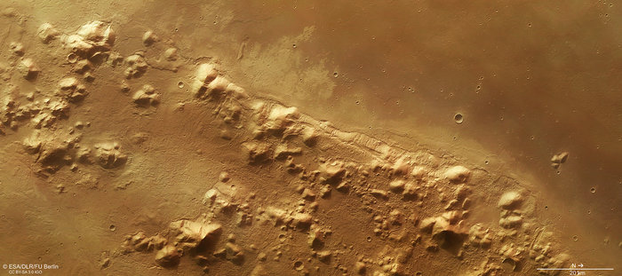
(ESA/DLR/FU Berlin, CC BY-SA 3.0 IGO)

Also, watch the following footage by ESA, which shows a wonderful animation of Mars surface.

I hope you enjoyed this tutorial and of course, Happy April Fools' Day!