From GIS to Remote Sensing: Tutorial: Supervised Classification of Land Cover and Mosaic of Several Landsat images

This tutorial is about the land cover classification of several Landsat images in order to create a classification of a large study area using the Semi-Automatic Classification Plugin (SCP). For very basic tutorials see Tutorial 1: Your First Land Cover Classification and Tutorial 2: Land Cover Classification of Landsat Images.

The study area of this tutorial is Costa Rica , a Country in Central America that has an extension of about 51,000 square kilometres. In particular, we are going to classify Landsat 8 and Landsat 7 images, masking clouds and creating a mosaic of classifications. We are going to identify the following land cover classes:

Built-up;
Vegetation;
Soil;
Water.

Following the video of this tutorial.

Plugin installation

First, install the SCP. For information about the installation of QGIS in various systems see Plugin Installation.

Open QGIS; from the main menu, select Plugins > Manage and Install Plugins;

From the menu All, select the Semi-Automatic Classification Plugin and click the button Install plugin;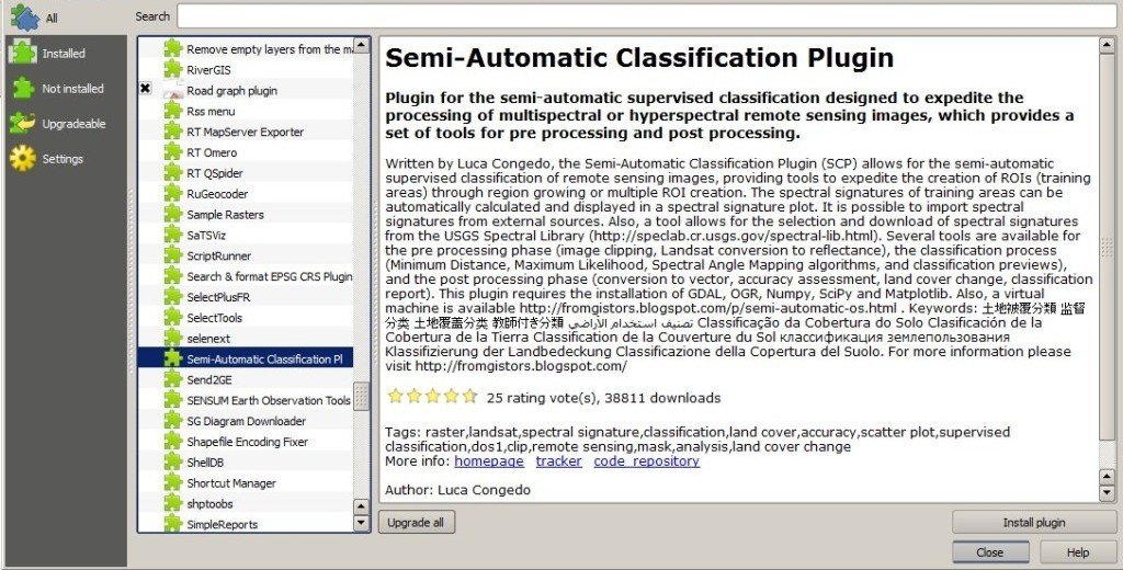

The SCP should be automatically activated; however, be sure that the Semi-Automatic Classification Plugin is checked in the menu Installed (the restart of QGIS could be necessary to complete the SCP installation);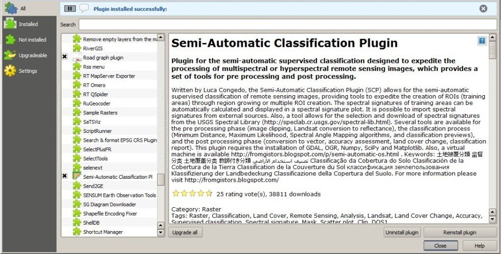

We are going to set some of the SCP options in order to optimize the following processes. Open the Settings clicking the button

and select Settings: Processing. Now, in Classification process check the options Use virtual rasters for temp files and Raster compression, in order to save disk space during the processing.

In RAM set the available RAM (in MB) for processing entering half of the system RAM; for instance it your system has 2GB of RAM enter 1024. If the system is 32bit, due to system limitations you should not enter values higher than 512MB.

SCP settings

In order to ease the photo interpretation in the following steps, we are going to use also the OpenLayers Plugin which allows for the display of several maps. If you don’t have already installed, follow the same steps previously described and install the OpenLayers Plugin in QGIS.

Download and Pre processing of Landsat images

We are going to download Landsat 7 and 8 images using the SCP tool Download Landsat. Landsat images are available from the U.S. Geological Survey, and these bands are downloaded through the Google Earth Engine and the Amazon Web Services. Also, we are going to convert Landsat images to reflectance and apply the DOS1 atmospheric correction (see Landsat image conversion to reflectance and DOS1 atmospheric correction).

First, we need to download the Landsat database in SCP. Open the tab Download Landsat clicking the button

in the SCP menu or the Toolbar. Click the button Select database directoryin order to define where to save the database. It is preferable to create a new directory (e.g. LandsatDB) in the user directory. Click the button Update database and click Yes in the following question about updating the image database.

TIP : Landsat databases are updated daily, therefore when you need up to date images you should click the button Update database in order to the get the latest Landsat images.

Landsat database download

Now we could define the Area coordinates of the study area, click Find images and browse Landsat images. Each Landsat image has a unique ID (i.e. identifier). In this tutorial we are going to use two Landsat 8 images acquired on February 2014 (IDs: LC80150532014050LGN00 and LC80160532014057LGN00) and a Landsat 7 image acquired on March 2014 (ID: LE70150532014090EDC00); of course, more images are required for the classification of the whole Country.

With SCP, it is possible to find an image basing on the ID thereof using the Search options. In particular, in Image ID paste the following IDs and click Find images:

LC80150532014050LGN00; LC80160532014057LGN00; LE70150532014090EDC00

After a few seconds, the three images are listed in the Landsat images.

Landsat image search

Before downloading the images, we need to define the options for the conversion to reflectance which will be performed automatically to downloaded images. Open the tab Landsat clicking the button

in the Toolbar ; enable the options Apply DOS1 atmospheric correction and Brightness temperature in Celsius. Also, leave checked Use NoData value (image has blackborder).

TIP : check Perform pan-sharpening in order to perform the Pan-sharpening of Landsat images producing bands with 15m spatial resolution; of course, using pan-sharpened images increases the classification time (because a greater number of pixels need to be processed) and can increase the spectral variability.

Landsat pre processing

Now, open the tab Download Landsat and uncheck the options only if preview in Layers and Load bands in QGIS (leave checked Pre process images in order to convert bands to reflectance automatically). Click the button Download images from list to select an output directory and start the download process (this may take a while).

Landsat download

When the download process is finished, several directories are created in the output directory with the name like Landsat ID, containing the original Landsat bands and the converted bands (with the suffix _converted).

Classification of Landsat Images

We are going to start the classification of the Landsat 8 image LC80150532014050LGN00 converted to reflectance. Open the directory LC80150532014050LGN00_converted.

In QGIS, open the following bands (also with drag and drop):

RT_LC80150532014050LGN00_B2.tif = Blue;

RT_LC80150532014050LGN00_B3.tif = Green;

RT_LC80150532014050LGN00_B4.tif = Red;

RT_LC80150532014050LGN00_B5.tif = Near-Infrared;

RT_LC80150532014050LGN00_B6.tif = Short Wavelength Infrared 1;

RT_LC80150532014050LGN00_B7.tif = Short Wavelength Infrared 2.

Open the tab Band set clicking the button

in the SCP menu or the Toolbar. Click the button Select All, then Add rasters to set, and then Sort by name for ordering bands automatically. Finally, select Landsat 8 OLI from the combo box Quick wavelength settings, in order to set automatically the center wavelength of each band (this is required for the spectral signature calculation).

TIP : click the button Build band overviews in order to improve display performance of bands.

Definition of Band set

In the list RGB select the item 4-3-2 for displaying a Color Composite of Near-Infrared, Red, and Green. A temporary virtual raster of the Band set will be created in QGIS, allowing for the photo interpretation of the image.

Now we need to create Training shapefile and Signature list file in order to collect Training Areas (ROIs) and calculate the Spectral Signature thereof (for very basic definitions see Tutorial 1: Your First Land Cover Classification).

In the ROI Creation dock click the button New shp and define a name (e.g. ROI.shp ) in order to create the Training shapefile that will store ROI polygons. The shapefile is created and added to QGIS. The name of the Training shapefile is displayed in Training shapefile .

Also, click the button Save in the Classification dock and define a name (e.g. SIG.xml ) in order to create the Signature list file that will store spectral signatures. The path of the Signaturelist file is displayed in Signature list file .

Definition of SCP input for the Landsat image LC80150532014050LGN00

Now we are ready for the creation of ROIs. We are going to use the same codes for ROIs in all the Landsat images, according to the following table.

Macroclass name	Macroclass ID
Built-up	1
Vegetation	2
Soil	3
Water	4

About the basics of ROI creation see Create the ROIs. It is possible to create ROIs by drawing manually a polygon using the button

or with region growing pressing the button + and then clicking the map. Use the button

in ROI creation for zooming to the polygon extent of the ROI, and Show for showing or hiding the temporary ROI.

Example of Built-up ROI

Example of Vegetation ROI

Example of Soil ROI

Example of Water ROI

With the ROI Creation dock create as many ROIs as possible, assigning a unique Class ID (C_ID) to each ROI, and the Macroclass ID (MC_ID) of the corresponding Macroclass. If Displaycursor for is checked in the ROI creation, the NDVI value of the pixel beneath the cursor is displayed in the map: it is useful for detecting vegetation pixels (characterized by high NDVI values).

TIP : change frequently the Color Composite and use the buttons and in the Toolbar for stretching the minimum and maximum values of the displayed image; also, use the button Show for hiding and showing the image.

ROIs are used for the calculation of spectral signatures that are used by the classification algorithm in order to classify the entire image. In this tutorial we are going to use the Maximum Likelihoodalgorithm.

After the creation of each ROI it is useful to check the Spectral Distance in order to assess the separability of ROI; in fact, each ROI should be different (i.e. spectrally distant) from the others, in order to avoid spectral confusion and achieve better classification results.

In the Signature list highlight the ROIs and click the button

. Spectral signature are added to the Spectral Signature Plot.

Plot of spectral signatures

Now click the tab Spectral distances. Each table represent the Spectral Distance of each ROI combination.

As shown in the following figure, the comparison of the Built-up ROI and the Soil ROI highlights very low Spectral Angle and Euclidean Distance; this means high similarity if we used the Spectra Angle Mapping or the Minimum Distance algorithms. The Jeffries-Matusita Distance is near 2; this means that the two ROIs are separable for the Maximum Likelihood algorithm.

Since we are using the Maximum Likelihood algorithm, it is important that the Jeffries-Matusita Distance is near 2 for each ROI combination.

Spectral distances

Now we can create a classification preview (see Create a Classification Preview for the basics of classification previews).

In the Classification algorithm select the classification algorithm Maximum Likelihood. In Classification preview set Size = 500 , click the button + and then left click in the map in order to create a classification preview. Use the Transparency tool for changing the preview transparency and display the classification over the image.

Classification preview

In the Classification algorithm, click the button + and then right click in the map for calculating the algorithm raster. The algorithm raster represents the calculation result of the Classification Algorithms; it is useful for locating where we need to create new ROIs.

As shown in the following figure, the algorithm raster has a grey scale symbology, where dark areas represent pixels that the algorithm found distant from all the spectral signatures and white areas represents pixels that are very similar to spectral signatures. In these dark areas we have a greater level of uncertainty, therefore we need to create new ROIs in order to improve the classification results.

Preview of the algorithm raster

We can notice the presence of clouds in the image. In order to avoid classification errors, we need to mask clouds.

There are several methods for masking clouds; during the classification step, a simple method for masking clouds is the creation of ROIs. Create a new ROI inside a cloud in the image, and assign a unique Class ID and the Macroclass ID equals to 0. In fact, the MC ID = 0 is used by SCP for the category Unclassified, which means that cloud pixels are not classified (i.e. masked).

ROI created for cloud masking

In the following image, we can see that clouds are now masked. However, pixels near the border of clouds are classified incorrectly as Built-up. In the next paragraphs, more effective methods are described for masking clouds after the classification process (see Cloud Masking).

Classification preview over clouds

TIP : load a service such as OpenStreetMap using the OpenLayers Plugin, which can ease the photo interpretation and the ROI creation.

OpenStreetMap loaded in QGIS

When we are happy with the results of the previews, we can perform the classification of the whole image. In Classification algorithm, activate the checkbox Use Macroclass ID. In theClassification output click the button Perform classification and define the name of the classification output (e.g. classification_1.tif).

Land cover classification 1 of the Landsat image LC80150532014050LGN00

We can see that part of the clouds are black (i.e. unclassified), however several cloud pixels are classified as Built-up. Also, the black border of the Landsat image is classified as Built-up. We are going to correct these errors and refine the classification in the next steps.

Now, in QGIS open the following Landsat 8 bands that are inside the directory LC80160532014057LGN00_converted.

RT_LC80160532014057LGN00_B2.tif = Blue;

RT_LC80160532014057LGN00_B3.tif = Green;

RT_LC80160532014057LGN00_B4.tif = Red;

RT_LC80160532014057LGN00_B5.tif = Near-Infrared;

RT_LC80160532014057LGN00_B6.tif = Short Wavelength Infrared 1;

RT_LC80160532014057LGN00_B7.tif = Short Wavelength Infrared 2.

Repeat the above steps for the creation of the Band set, the Training shapefile and Signature list file.

TIP : close QGIS and create a new QGIS project for each Landsat image, in order to delete temporary files and free disk space.

Definition of SCP input for the Landsat image LC80160532014057LGN00

Create a land cover classification repeating the steps previously described.

Land cover classification 2 of the Landsat image LC80160532014057LGN00

In a new QGIS project, open the Landsat 7 bands inside the directory LE70150532014090EDC00_converted:

RT_LE70150532014090EDC00_B1.tif = Blue;

RT_LE70150532014090EDC00_B2.tif = Green;

RT_LE70150532014090EDC00_B3.tif = Red;

RT_LE70150532014090EDC00_B4.tif = Near-Infrared;

RT_LE70150532014090EDC00_B5.tif = Short Wavelength Infrared 1;

RT_LE70150532014090EDC00_B7.tif = Short Wavelength Infrared 2.

You can see that this image covers the same area as the Landsat 8 image LC80150532014050LGN00. In fact, we are going to use the classification of this Landsat 7 image in order to fill the Unclassified pixels of the Landsat 8 image.

Definition of SCP input for the Landsat image LE70150532014090EDC00

Again, create a land cover classification following the steps previously described.

Land cover classification 3 of the Landsat image LE70150532014090EDC00

Now, we have 3 land cover classifications that we can enhance in several ways.

Enhancement of Classification Using NDVI

We are going to calculate NDVI for enhancing the classification using the Band calc (see Tutorial: Using the tool Band calc). In particular, pixels where NDVI value is above a certain threshold will be classified as vegetation (code 2). Below this NDVI threshold, the Maximum Likelihood classification is untouched.

Of course, this is an example of integration of ancillary data; we could use other data such as other vegetation indices or the result of other classifications (e.g. using Spectra Angle Mapping).

Now, in QGIS load the bands of the Landsat 8 image LC80150532014050LGN00 and the respective land cover classification. Open the Band calc and click the button Refresh list. In the Band calc, calculate the NDVI copying the following Expression:

("RT_LC80150532014050LGN00_B5" - "RT_LC80150532014050LGN00_B4")  /  ("RT_LC80150532014050LGN00_B5" + "RT_LC80150532014050LGN00_B4")

Click the button Calculate, select where to save the NDVI (e.g. a new file named NDVI_1.tif).

NDVI calculation

Then, calculate the following Expression for enhancing the classification basing on the NDVI:

np.where("NDVI_1" > 0.6, 2, "classification_1")

Click the button Calculate, and select where to save the new classification (e.g. classification_1_NDVI.tif). We can see in the following figure that the area classified as vegetation has increased.

Classification 1 refined with NDVI

In this case we have used a NDVI threshold equals to 0.6 . However, the threshold value has to be chosen for every image, because NDVI can vary from image to image.

Now we perform the same enhancement for the other land cover classifications. For the Landsat 8 image LC80160532014057LGN00 calculate NDVI with the following expression:

("RT_LC80160532014057LGN00_B5" - "RT_LC80160532014057LGN00_B4")  /  ("RT_LC80160532014057LGN00_B5" + "RT_LC80160532014057LGN00_B4")

and the following expression for enhancing the classification:

np.where("NDVI_2" > 0.5, 2, "classification_2")

Classification 2 refined with NDVI

For the Landsat 7 image LE70150532014090EDC00 calculate NDVI with the following expression:

("RT_LE70150532014090EDC00_B4" - "RT_LE70150532014090EDC00_B3")  /  ("RT_LE70150532014090EDC00_B4" + "RT_LE70150532014090EDC00_B3")

and the following expression for enhancing the classification:

np.where("NDVI_3" > 0.5, 2, "classification_3")

Classification 3 refined with NDVI

Now that the classification of vegetation has been enhanced for the three images, we are going to mask clouds and border pixels in order to avoid classification errors.

Cloud Masking

Landsat 8 images include Quality Assessment bands (QA) that are useful for identifying clouds. Pixel values of QA bands are codes that represent combinations of surface and atmosphere conditions. These values indicate with high confidence cirrus or clouds pixels (for the description of these codes see the table at http://landsat.usgs.gov/L8QualityAssessmentBand.php ).

The QA band of the Landsat 8 image LC80150532014050LGN00 includes mainly the values 53248 and 61440 indicating clouds, and the value 36864 indicating potential clouds. Therefore, we are going to write an expression that masks our classification (i.e. classification_1_NDVI) where pixels of the QA band are equal to one of these values.

In QGIS, open the band LC80150532014050LGN00_BQA that is inside the directory LC80150532014050LGN00 of the downloaded Landsat image and the classification_1_NDVI. Copy the followingExpression in the Band calc:

np.where(("LC80150532014050LGN00_BQA" == 53248) | ("LC80150532014050LGN00_BQA" == 36864) | ("LC80150532014050LGN00_BQA" == 61440), 0, "classification_1_NDVI")

Click the button Calculate, and select where to save the new classification (e.g. classification_1_clouds.tif).

Classification 1 with masked clouds

Clouds are almost completely masked (i.e. Unclassified); however, some pixels are still classified as Built-up (in red). We can do the same for the image LC80160532014057LGN00 using the following Expression in the Band calc:

np.where(("LC80160532014057LGN00_BQA" == 53248) | ("LC80160532014057LGN00_BQA" == 36864) | ("LC80160532014057LGN00_BQA" == 61440), 0, "classification_2_NDVI")

The Landsat 7 image does not have the QA band. Another method for masking clouds uses the Blue and the Thermal Infrared (converted to temperature) bands, basing on the fact that clouds are generally colder than soil and have high reflectance values in the blue band. Landsat 7 is also affected by black stripes (i.e. SLC-off) that we are going to mask as well.

We are going to create an expression that identifies pixel values below a certain temperature threshold for the Thermal band (band 6 for Landsat 7), and above a certain reflectance threshold for the Blue band (band 1).

In QGIS load all the Landsat bands inside the directory LE70150532014090EDC00_converted. Use the following expression in the Band calc:

np.where((("RT_LE70150532014090EDC00_B6_VCID_1"<23) & ("RT_LE70150532014090EDC00_B1">0.1)) | ("RT_LE70150532014090EDC00_B1" == 0) | ("RT_LE70150532014090EDC00_B2" == 0) | ("RT_LE70150532014090EDC00_B3" == 0) | ("RT_LE70150532014090EDC00_B4" == 0) | ("RT_LE70150532014090EDC00_B5" == 0) | ("RT_LE70150532014090EDC00_B7" == 0), 0,"classification_3_NDVI")

The first part (("RT_LE70150532014090EDC00_B6_VCID_1"<23) & ("RT_LE70150532014090EDC00_B1">0.1)) means that we are going to mask pixels that have both temperature lower than 23°C and Blue band reflectance greater than 0.1 . These threshold values have been identified in the image, using the tool Identify of QGIS for cloud pixels in band 1 and band 6.

The character | means or , so that the other expressions (e.g. "RT_LE70150532014090EDC00_B1" == 0) identify pixel values equal to 0 (which are NoData) for every Landsat band, in order to mask the black stripes due to SLC-off and the black border.

Classification 3 with masked clouds

We could use the same method of cloud masking also for Landsat 8 images. For the image LC80150532014050LGN00 load the bands RT_LC80150532014050LGN00_B10 andRT_LC80150532014050LGN00_B2, and use the following Expression in the Band calc:

np.where((("RT_LC80150532014050LGN00_B2" > 0.03) & ("RT_LC80150532014050LGN00_B10" < 24)) | ("RT_LC80150532014050LGN00_B2" == 0), 0, "classification_2_NDVI")

The condition "RT_LC80160532014057LGN00_B2" == 0 allows for the masking of the image black border.

Classification 1 with clouds masked using the alternative method

As you can see, there are still gaps (Unclassified pixels) in the classification; we would require the classification of other Landsat images in order to fill those gaps. After the cloud masking of these three classifications, we can create one mosaic that is the classification of the whole study area.

Part of the unclassified gaps has been filled with the Landsat 7 classification. Of course, we would require more classifications in order to fill all the gaps.

Mosaic of Classifications

In order to create a mosaic of classifications, we are going to write an expression that will fill Unclassified pixels of the Landsat 8 image (ID LC80150532014050LGN00) with the classification of the Landsat 7 image (ID LE70150532014090EDC00). Also, we are going to merge these classifications to third one (the Landsat 8 image with ID LC80160532014057LGN00).

In QGIS open the three cloud masked classifications. Copy the following Expression in Band calc:

np.where("classification_1_clouds" == 0,  np.where("classification_3_clouds" == 0, "classification_2_clouds", "classification_3_clouds"), "classification_1_clouds")

Uncheck the checkbox Intersection in Output raster and click Calculate. The result (e.g. classification_mosaic) is shown in the following image.

Classification mosaic

In the following steps we are going to perform the accuracy assessment and the estimation of land cover area.

Accuracy Assessment

Accuracy Assessment is an important step of a land cover classification. In this tutorial we are going to use the Training shapefile as reference for assessing classification accuracy. However, there other methods that can improve the validation reliability (see http://fromgistors.blogspot.com/2014/09/accuracy-assessment-using-random-points.html ).

In QGIS, load the classification mosaic and the Training shapefile used for the image LC80150532014050LGN00. In SCP open the tab Accuracy and click the buttons Refresh list. Selectclassification_mosaic as the classification to assess and the Training shapefile as reference shapefile. Also, select MC_ID as Shapefile field. Click Calculate error matrix and choose the output destination (e.g. accuracy.tif).

The process produces an error matrix and an error raster which are useful for assessing the quality of our classification.

Accuracy assessment

Clip of the Classification

Before calculating the area of each land cover class, we need to clip the classification to the extent of the study area, which is Costa Rica.

Download the Shapefile of Sub-National Administrative Units of Costa Rica from http://data.fao.org/map?entryId=c7a0f990-88fd-11da-a88f-000d939bc5d8&tab=metadata (clicking the Download button) by the FAO .

Extract the downloaded file (1173.zip) and load the shapefile costa rica.shp in QGIS (select WGS84 as projection).

The shapefile of Costa Rica by FAO

In this case, we need to define the projection of this shapefile. In QGIS, open the command Vector > Data management tool > Define current projection; select the shapefile costa rica asInput vector layer and choose EPSG:4326 - WGS 84 as spatial reference, and click OK.

Define the shapefile projection

Now we can clip the classification_mosaic.tif. Load the classification in QGIS. Open the command Raster > Extraction > Clipper. Select the classification_mosaic as input raster; set the output file (e.g. classification_clip.tif), and set No data value equals to 0. In Clipping mode enable Mask layer and select costa rica, then click OK.

Clipping the classification

Finally, we have a classification clipped to the extent of Costa Rica (as you can see we would need other classifications for covering the whole extent of Costa Rica), and we can calculate the classification report.

The clipped classification

Classification Report

In SCP open the tab Classification report and click the buttons Refresh list. Check Use NoData value setting the value equals to 0 and click the button Calculate classification report. The classification report is displayed with the count of pixels, the area, and percentage of each land cover class. You can save the report to text file clicking the button Save report to file.

Classification report

We have completed this tutorial about the land cover classification of a large area, using multiple Landsat images and creating a classification mosaic. It is worth pointing out that classification results depend on the season of the images. Therefore, the input images should be acquired in the same period, in order to avoid differences due for instance to the phenological state of vegetation or occurred land cover change.